Visualize Data

DeltaTwin® service is engineered to automatically analyze uploaded data resources and apply the most appropriate visualization method based on the file type and content structure. This process facilitates immediate data inspection without requiring any complex setup.

Visualizations are categorized into three primary types: textual, geospatial, raster/image. The following sections detail the logic, supported formats, and rendering methods for each category.

Interactive Geospatial Visualization

DeltaTwin® provides a robust solution for the visualization of geospatial data. Resources/Artifacts identified as containing geographic information are rendered as interactive layers on a deck.gl map. This visualization is automatically triggered for any resource containing recognizable geographic data.

Supported Formats

• GeoJSON and KML: These standard vector formats are natively supported. All geometric features (e.g., points, linestrings, polygons) contained within these files are parsed and rendered on the map interface.

• CSV & JSON: For tabular or structured data, DeltaTwin® automatically scans for column headers or keys like latitude, longitude, lat, or lon. If found, it will plot each entry as a point on the map. Users still have the option to select the appropriate column header or JSON path that corresponds to the latitude or longitude data.

This feature is perfect for visualizing sensor locations, GPS tracks, administrative boundaries, and more.

Image & Scientific Data Visualization

For binary data, seeing the resource is key. DeltaTwin® provides a direct and clear rendering for a range of standard and scientific image formats.

Supported Formats

• Standard Images: You can instantly view common image files like PNG, JPEG, and GIF.

Text-Based Data Viewer

Not all data is visual, but it still needs to be readable. For any file that can be interpreted as text, DeltaTwin® provides a formatted, and syntax-highlighted viewer (where applicable). This is the default visualization for any format not rendered as a map or an image.

This is perfect for quickly inspecting:

• Structured Data: JSON, XML
• Tabular Data: CSV (as raw text)
• Plain Text: TXT and any other unrecognized text-based format. This allows you to examine raw data sources directly within the service interface, eliminating the need for external software or file downloads for preliminary analysis.

Map layers in DeltaTwin®

DeltaTwin® leverages deck.gl layers to provide rich, interactive visualizations for geospatial resources/artifacts. Layers define how data is represented on the map, whether as points, grids, heatmaps, or shapes. Choosing the right layer type helps highlight different aspects of your data, from density patterns to categorical distributions.

Supported Layers

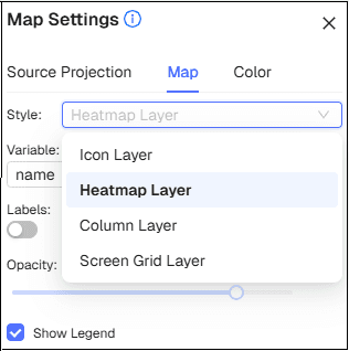
DeltaTwin® currently supports five deck.gl layers:

GeoJsonLayer

This layer displays vector geometries such as points, lines, and polygons. It is is the default and only layer used for GeoJSON and KML formats as it preserves the full geometry structure (boundaries, paths, markers).

HeatmapLayer

Heatmaps are an excellent use case for visualizing the density of geospatial points from CSV or JSON datasets that contain latitude/longitude fields. This technique is highly effective for identifying hotspots and areas with high event frequency (like accidents or the availability of electric bike stands in stations), as it quickly highlights clusters and intensity without the clutter of displaying every individual point.

ColumnLayer

The ColumnLayer is a suitable visualization technique to represent numerical values as 3D columns at given coordinates. It applies to CSV or JSON datasets containing latitude, longitude, and a numeric attribute. For instance, it can visualize population by district (where the column’s height equals the population) or represent production output tied to specific locations. The key advantage of the ColumnLayer is that it adds a dimensional aspect to the data, which makes it easy to compare values spatially.

IconLayer

The IconLayer is used to represent geospatial points with custom icons, applicable to CSV or JSON datasets containing latitude and longitude fields. Its use cases include distinguishing between categories or providing clear markers for incidents, facilities, or assets (using different icon colors for air quality stations owners/agencies, or the method used for water level observations). The primary advantage of the IconLayer is that it enhances interpretability by directly associating a visual symbol with the data’s category or meaning.

ScreenGridLayer

The ScreenGridLayer aggregates massive point datasets into a density heat-map based on screen-space pixels, not geographic coordinates. It divides the visible area into fixed-size cells, calculating a sum or count of data points within each, allowing for immediate, clear identification of hotspots and concentration patterns in use cases like analyzing rideshare demand or traffic density.

How Visualization Works

When creating a resource or saving an artifact, automatic format detection ensures that the data type is recognized correctly.

• Tabular and structured files are shown in formatted text.
• Geospatial data is visualized on a map.
• Image and raster files are displayed directly in the viewer.

Map, Interactive map exploration

Loading data

We start by loading the geospatial features from the input resource/artifact on the Map tab. Since GeoJSON and KML are standard formats, the map can automatically load and visualize them without any extra steps or the user having to select specific features.

As for generic CSV and JSON data, which we do not follow any standard, we ask the user to select which CSV columns or JSON keys hold the geospatial features. These features can either be a separate latitude and lontigude columns/keys, or the they can be combined in one column/key (ex: [48.838047917889284, 2.590412928851182]).

After selection, the map will display the data, and generates a legend to explain the resulting color coding. The content and style of the legend are determined by the data type of the selected variable. If the variable is numerical (e.g., measurements or predictions), the legend displays a smooth color gradient from the chosen palette, clearly marking the minimum and maximum values found in the data. If the variable is textual or categorical (e.g., names or status), the legend presents up to ten distinct, arbitrarily selected values from the variable, each assigned a unique color, allowing users to quickly correlate categories with their corresponding visual representation on the map. The user can also select which variable will be assotiaced as a label of the points on the map.

Showing data on the map

We suppose that most artifacts/resources (CSV, JSON, KML, GeoJSON) hold key properties that represent real-world information (measurements, categories, predictions, etc.). To visualize this data effectively, DeltaTwin® prompts you to choose one “Variable” that will drive the map’s appearance. Upon selection, the interface instantly recolors map elements (point/polygon/line/marker color, or column elevation, heatmap) to reflect the value distribution of your chosen property. For CSV and JSON points, DeltaTwin® also prompts the user to variable that holds the label of each point on the map.

The Tooltip tab gives the user control over the interactive information displayed when hovering over data points on the map.

The user is prompted to select a specific variable from their resource/artifact. The values from this chosen variable will then be displayed as a tooltip, providing immediate context and details whenever the user interacts with a feature on the visualization.

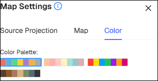
Color

The Color tab provides users with simple options for styling data visualization on the map. It offers five predefined color palettes, allowing you to quickly select a color series that best suits your data or aesthetic preference, instantly applying the chosen color scheme to the features displayed on the map.

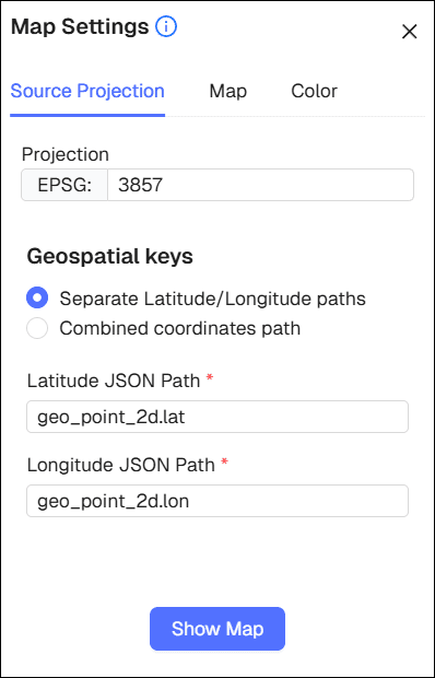
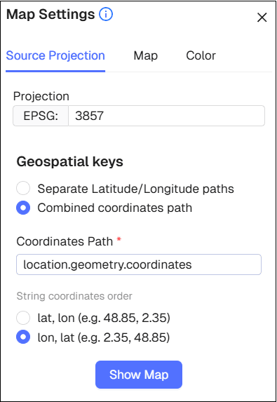
Source Projection

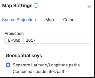
Coordinate reference system (CRS projection)

Geospatial keys (Latitude and longitude values)

For CSV and JSON files, you must indicate how to read the latitude and longitude values.

• When you upload a CSV file, you’ll need to tell us which column holds the latitude and which column holds the longitude. If both are stored together in one column (separated by a comma or space), just check the “Combined coordinates field” box and pick the column with the combined coordinates.
• For JSON files, just enter the dot-notation path to the fields that store latitude and longitude values. By default, there are assummed to be in separate fields. However, if both are stored together in one field (like ‘coordinates’ or ‘location’), then select the “Combined coordinates path” option and enter the dot path to that combined field.

For example, if a JSON object is structured as

[
  {
    "@iot.selfLink": "https://airquality-frost.k8s.ilt-dmz.iosb.fraunhofer.de/v1.1/Locations(1)",
    "@iot.id": 1,
    "name": "STA.09.LIES",
    "description": "Location of station STA.09.LIES",
    "encodingType": "application/geo+json",
    "location": {
      "type": "Feature",
      "properties": {},
      "geometry": {
        "type": "Point",
        "coordinates": [10.0080800000001, 53.57392]
      }
    },
    "properties": {
      "AirQualityStationArea": "suburban",
      "countryCode": "AT",
      "localId": "STA.09.LIES",
      "metadata": "http://discomap.eea.europa.eu/map/fme/metadata/PanEuropean_metadata.csv",
      "namespace": "AT.0008.20.AQ",
      "owner": "http://dd.eionet.europa.eu "
    }
  }
]

the (combined) latitude/longitude can be accessed using the path location.geometry.coordinates, which would return the value [10.0080800000001, 53.57392]. Furthermore, you can specified string coordinates order ( “lat, lon” or “lon”, “lat”).

Example:

Similarly, you would use geo_point_2d.lon and geo_point_2d.lat to extract latitude and longitude from this json:

[
  {
    "datetime": "2025-10-01T10:52:00+02:00",
    "predefinedlocationreference": "10273_D",
    "averagevehiclespeed": 74,
    "traveltime": 10,
    "traveltimereliability": 75,
    "trafficstatus": "freeFlow",
    "vehicleprobemeasurement": 2,
    "geo_point_2d": {
      "lon": -1.6502152435538264,
      "lat": 48.044792756860865
    },
    "gml_id": "rva_troncon_fcd_v1_1.5458",
    "id_rva_troncon_fcd_v1_1": 5458,
    "hierarchie": "R\u00e9seau d'armature",
    "hierarchie_dv": "R\u00e9seau de transit",
    "denomination": "Route d\u00e9partementale 34",
    "insee": 35206,
    "sens_circule": null,
    "vitesse_maxi": 70
  }
]

Example: